The measurement of electoral history 1994–2018

(Versión en español aquí.)

This note presents, discusses, and distributes statistics (available here) of party electoral performance in Mexico's competitive era. It elaborates two quantities of interest: voting forecasts based on recent electoral history and measures of parties' core support. The procedure generates summary measures of recent electoral history in relatively small geographic units, municipalities (\(N \approx 2500\)) and secciones electorales (\(N \approx 66000\)) throughout Mexico. I apply the procedure to four federal congressional elections between 2009 and 2018, using results since 1994 as historical input.

The note starts by showing the statistics in action to get a glimpse of their descriptive and analytic potential. By summarizing recent electoral history and its geography, the quantities offer a scenic view of a critical aspect of contemporary Mexican politics.

Later sections offer methodological detail on the estimation of these quantities of interest and are increasingly technical.

1. Statistics in action

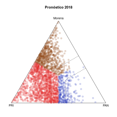
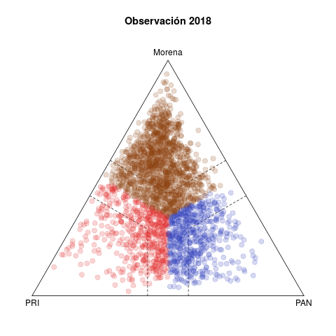
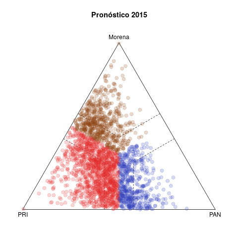
Table 1 presents two pairs of diagrams for the 2015 (below) and 2018 (above) congressional elections. Each dot represents one municipality, colored according to the winning party, with coordinates in the ternary plot according to the relative votes of the PAN, the PRI, and the left in the federal deputy race (other smaller parties are excluded).¹

Table 1: Historic expectations and municipal-level vote in two congressional elections

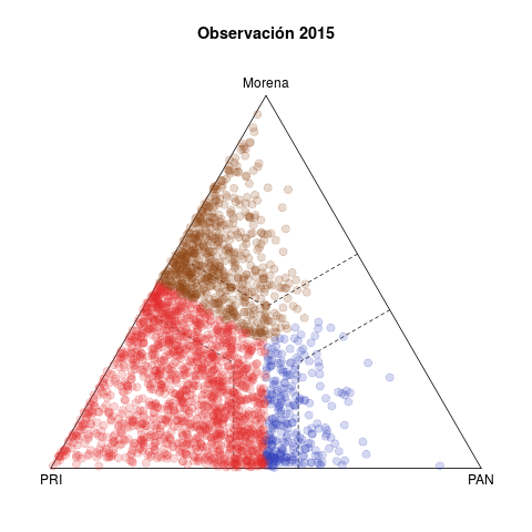The left side shows the vote forecasts. The idea behind this statistic is summarizing the evolution of relative votes in the municipality in five previous elections (2003–2015 in the case of 2018) and using the trend to project a vote forecast for the current year. Plots in the right side show the actual results observed in both elections.

Three features are noteworthy in 2018. The first is the discrepancy between the left and right plots. Either the model does a poor job forecasting, or 2018 was an extraordinary election. History gave license to expect a comfortable PRI victory, both in the number of municipalities won and in margins of victory. Municipalities outside the dotted bands are won by margins of 15 points or more, and the bulk of secure municipalities are red in the forecast, with Morena in a distant second place. In fact, although a significant number of municipalities migrated towards the PAN, it was Morena who showed a clear advantage. PRI was the underachiever. In contrast, the lower left and right plots reveal fewer differences between them—2015 was a more normal election, the past offering much better grounds to forecast.

Second, observed municipalities fled the edges and triangle vertices in 2018. Observations in vertices show a party that has no significant challenger. While those on the edges were bipartisan, whether more (inside dotted bands) or less (outside the bands) symmetric. It is also plain in forecasts that only the PAN–Morena edge was expected to be unpopulated. In practice, however, third party vote rarely collapsed to zero, there was much more dis-coordination than in the past. In fact, the intersection of dotted bands appeared denser and more homogeneous in the right than the left diagram.

Third, the PAN vs left competition was legal tender in 2018. The pattern in competitive municipalities in the last two decades, still visible in the 2015 plots, involved either PRI–PAN or PRI–left rivalries, and rarely PAN–izquierda. It was this pattern that eased electoral alliances between PAN and PRD in sub national races since 2010 that culminated in the Frente they formed in 2018 to nominate a joint presidential candidate.

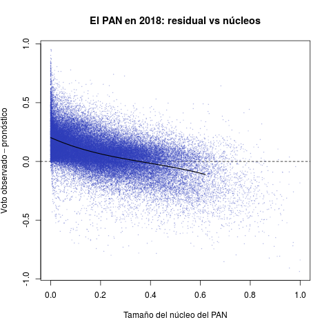
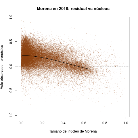
Plots in Table 2 report secciones electorales and therefore offer much finer-grained than the previous portraits. They introduce the other quantity of interest in this note: parties' core support. The idea behind this statistic is measuring the size of the group that has historically supported the party consistently, in good but also in bad years.

Table 2: Support core and party performance in 2018

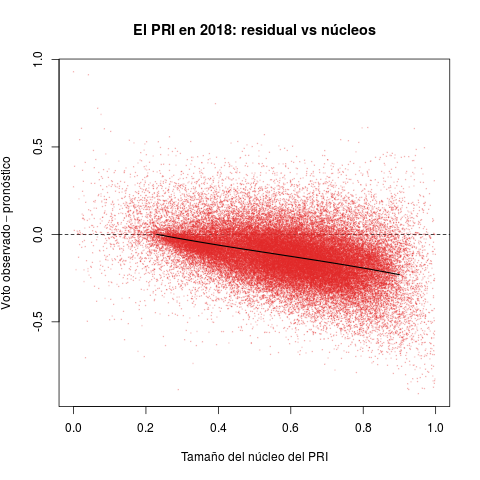The horizontal axis in each plot measures the size of party core support groups as a proportion of the sección's electorate. The PRI enjoyed a clear edge over the rest of the parties in the period, with sizable cores in all secciones nationwide. The distributions of the PAN and the left, in contrast, appear concentrated towards the zero—they have relatively few secciones with some unconditional support.

The vertical axis reports the three parties' performance in 2018 (the difference between the observed vote and the forecast). Positive values indicate that the party excelled expectations in the sección, negative ones that it under-performed it expectation. The PRI's electoral disaster appears all too clearly in the red plot. There were a few secciones with positive performance, but the density concentrates massively below the horizontal zero line, something that Table 1 had hinted. What is truly remarkable is that the dismal performance is directly proportional to the size of the PRI core. President Peña and candidate Meade achieved what seemed, if not impossible, extremely improbable: they alienated the PRI's unconditional voters in 2018. The PAN and the left met expectations in secciones where they have enjoyed with groups of support. Both (especially Morena) over-achieved where they lack important cores, taking away PRI voters.

The note elaborates how statistics were prepared (replication code can be found here).

2. First differences

One common approach to study electoral change is through first differences. Denoting \(v_t\) the party's vote share in the municipality or the sección, in period \(t\), the first difference is simply \(d_t = v_t - v_{t-1}\).

\(d_t\) is an intuitive quantity, showing the sign and magnitude of change from one election to the next. But, precisely because it compares pairs of consecutive elections only, it misses more dynamic processes in the units. One example, well documented by electoral sociology, is the regression to the mean (Campbell 1991, Segovia 1979). Detection requires observing the unit through at least three consecutive periods to verify contrary signs in \(d_{t+1}\) and \(d_t\). The study of secular change in the Mexican party system in the last quarter of century calls for deeper historical perspective.

(First differences appear in the fields d.pan, d.pri, and d.morena in the distributed data.)

3. The recent linear trend

One way of adopting it is with vote forecasting from trends discernible in the previous five congressional races (Magar 2012). I summarize the central tendency of the recent historical vote by means of linear estimation in time, fitting a straight line for each year analyzed and each party in the municipality or sección electoral.

The slope of the fitted line (the trend) serves to extrapolate the party's electoral support to the future. For instance, to get the vote share that the recent past predicts for a party in unit \(u\) for 2018, I estimate equation 1

\[v_{ut} = a + b \times t + \text{error}, \; t = 2003, \ldots, 2015\]

that I then use to predict \(\hat{v}_{u2018} = \hat{a} + \hat{b} \times 2018\). This is an out-of-sample prediction of the party's vote share, it can be compared to the party's actual vote share in 2018 to gauge whether or not the unit approximates the historical record. For the 2015 forecast the sample shifts one period to become \(t = 2000, \ldots, 2012\), and so on an so forth for previous years. I distribute forecasts for 2009, 2012, 2015, and 2018, which involved fitting about 10 thousand municipal regressions and more than 250 thousand sección-level.

(Vote forecasts appear in the fields vhat.pan, vhat.pri, and vhat.morena of the distributed data.)

4. The party's support core

The other historical statistic is the parties' core support in the unit. Its definition stems from classifying voters in three categories: (1) support groups, that in the past have consistently supported the party; (2) opposition groups, that have consistently supported another party; and (3) swing groups, that have neither consistently supported nor consistently opposed the party (Cox and McCubbins 1986). The party core consists of the support groups.

I use the procedure by Díaz Cayeros et al. (2016) to estimate this core. If \(\bar{v}_t\) denotes the party's mean support across all units in period \(t\),² for each party in each unit I fit equation 2 \[\begin{equation} v_{ut} = \alpha + \beta \times \bar{v}_t + \text{error}, \; t = 1994, \ldots, 2018. \end{equation}\] \(\beta\) measures the effect that national party tides have on the party's vote in unit \(u\). For instance, \(\hat{\beta}=1\) estimates that for every percentage point that the party wins or loses nationally in year \(t\), it also wins or loses one percentage point in the unit; \(\hat{\beta}=0\), on the other hand, would indicate the unit's full isolation form national swings. It is therefore a measure of party volatility in the municipality or sección (analogous to "beta volatility" in the financial literature).

The \(\alpha\) coefficient estimates the core size: expected support in unit \(u\) in the hypothetical case that the party receives no vote at the national level. For instance, \(\hat{\alpha}=.4\) would indicate that, in the starkest of scenarios, 40% of the electorate in the municipality is unconditional to the party—which would indeed be a core of substantial size.

A critique that can be anticipated towards this measure of the party's support core is its extreme counter-factual nature (King and Zeng 2006). It deserves rigorous scrutiny, something I plan doing in the near future.

(The parties' core support appears in the fields alphahat.pan, alphahat.pri, and alphahat.morena of the distributed data. Party volatility in betahat.pan, betahat.pri, and betahat.morena.)

5. Compositional variables

I close with an important feature of the model specifications, associated with the compositional nature of electoral returns. Compositional variables are quantitative descriptions of the parts of a whole. They therefore have two characteristics: they are (1) proportions that (2) add up to unity.³

When estimating parties separately, the challenge of equations 1 and 2 is to avoid forecasting vote shares less than zero or greater than one; and that the sum of party forecasts equals 1. To achieve this, Aitchison (1986) proposes substituting vote shares by log-ratios in the analysis. Arbitrarily setting the PRI as the reference party, define party \(p\)'s vote relative to the PRI as \[r_p = \frac{v_p}{v_{\text{pri}}}.\] A value \(r_p=1\) would indicate a tie between party \(p\) and the PRI, while \(r_p>1\) that \(p\) finished ahead of the PRI by a proportion given by the value of \(r_p\), and \(r_p<1\) that the PRI beat party \(p\).

Thus, equation 1 is re-specified as \[\ln r_{put} = a + b \times t + \text{error}\] y equation 2 as \[\ln r_{put} = \alpha + \beta \times \bar{r}_{pt} + \text{error}.\]

Applying the natural logarithm attenuates the effect of extreme regressor values on the dependent variable, similar as a logit regression would. Model fitting was done with ordinary least squares.

Log ratio estimates must be transformed to collect estimated party vote shares. Illustrating with a three-party case, it is trivial that

\begin{equation} \hat{v}_p = \frac{\hat{r}_p}{1 + \hat{r}_{\text{pan}} + \hat{r}_{\text{morena}}} \; \text{and} \; \hat{v}_{\text{pri}} = \frac{1}{1 + \hat{r}_{\text{pan}} + \hat{r}_{\text{morena}}.} \end{equation}

These are the quantities that the distributed data reports.

6. References

• Aitchison, John. 1986. The Statistical Analysis of Compositional Data. New York: Chapman and Hall.
• Campbell, James E. 1991. The presidential surge and its midterm decline in congressional elections, 1868-1988. The Journal of Politics 53(2):477-87.
• Cox, Gary W. and Mathew D. McCubbins. 1986. Electoral Politics as a Redistributive Game. The Journal of Politics 48(2):370-89.
• Díaz Cayeros, Alberto, Federico Estévez and Beatriz Magaloni. 2016. The Political Logic of Poverty Relief: Electoral Strategies and Social Policy in Mexico. New York: Cambridge University Press.
• King, Gary and Langche Zeng. 2006. The Dangers of Extreme Counterfactual. Political Analysis 14(2):131-59.
• Magar, Eric. 2012. Gubernatorial Coattails in Mexican Congressional Elections. The Journal of Politics 74(2):383-99.
• Segovia, Rafael. 1979. Las elecciones federales de 1979. Foro Internacional 20(3):397-410.

Footnotes:

¹

I must note that, for the left's electoral history (which I arbitrarily call "Morena" in the plots and distributed data), I systematically added up the votes of the PRD, PT, and MC up to 2015. I also added Morena's and PES's votes that year. In 2018 the left consisted of Morena, PT, and PES jointly.

²

The analyzed unit \(u\) should be dropped from period \(t\)'s mean in order to not include the dependent variable in the right side of the equation. I do not do this due to the large number of municipal or seccional units (each contributing a fraction to the mean) and the use of vote shares (so large units are watered down): this impact of this refinement should be negligible in each mean value.

³

Formally, the compositional are random variables subject to two constraints: \[0 \leq v_p \leq 1 \; \forall \; p \in P \; \;\] and \[\; \; \sum_P v_p = 1.\]