Estimation of inter-census quantities

A description and discussion of the procedure to project population data to non-census years.

Longitudinal analysis of elections is richer when socio-demographic controls are included, such as the share of indigenous language speakers or of households with earth floor in a unit. A key source of aggregate data is the census. Yet the mismatch between decennial censuses and the three-year election cycle is an obstacle. The census bureau fills the gap partially, distributing annual municipal projections of selected indicators only (see this for detail).

Systematic analysis of municipalities large and small (N ≈ 2500), of less common units such as federal or state electoral districts, or of much more disaggregated units like secciones electorales (N ≈ 67k) necessitates self-estimation of off-census socio-demographic indicators. This note discusses how I have achieved this, from official data, in the Recent Mexican Election Vote Returns repository.

1 Filling gaps through projection

I illustrate the problem with voting age population, one denominator to compute turnout rates. We need it in triennial federal elections from 1994 to 2021. In the period, the census bureau distributes population counts for 2000, 2010, and 2020—four "General Censuses"—and mid-decade counts in 1995 and 2005—two "General Counts".¹ From here on, `census' refers to counts and censuses indistinctly.

A geographic unit's population 18 years and older for non-census years can be projected, with inter- and extra-polation and with some assumptions, from the census figures available. Three approaches are inspected:

• line segments connecting each unit's contiguous pair of census points;
• a linear regression of census points for the unit on time; and
• a log-linear regression of the (log-transformed) points on time.

I compare the voting age population of municipalities generated by each.

2 Key assumptions

Projecting decennial or mid-decennial quantities yearly requires assumptions. Among them are the following:

1. Population counts, which are discrete variables, are modeled as continuous and differentiable. This in order to obtain slopes.
2. A demographic trend model underlies each approach: a straight procession in the segment and linear projections, curvilinear in the log-linear; fitting one trend for each pair of contiguous censuses in the segment approach, or a central trend for the unit from all the censuses in the other approaches.

3 Segments projection

In this approach, a given unit's population in any year is the population recorded in the previous census plus the yearly inter-census population change times the years since that census. Formally, if \(t_1, t_2, \dots\) are contiguous census years, a given unit's population for year \(t\) is:

\[\text{pop}_t = \left\lbrace\begin{aligned} & \text{pop}_{t_1} + \frac{\text{pop}_{t_2} - \text{pop}_{t_1}}{t_2 - t_1} \times (t - t_1) \; \; \text{for} \; t \in [t_1,t_2] \\ & \text{pop}_{t_2} + \frac{\text{pop}_{t_3} - \text{pop}_{t_2}}{t_3 - t_2} \times (t - t_2) \; \; \text{for} \; t \in [t_2,t_3] \\ & \dots \end{aligned}\right.\]

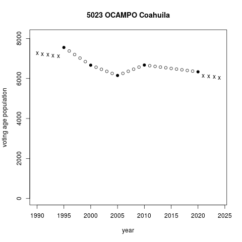
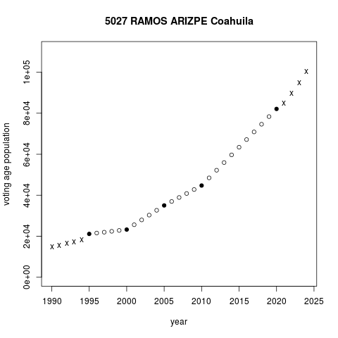
The plots below illustrate segments projection in two municipalities in the northern state of Coahuila. Ocampo municipality lost voting age population steadily in the period. Pay attention to circles in the plot only, black are census values, white are segments projections. The drop decelerated after a partial recovery in 2005-2010. Fitting separate straight segments for each inter-census period accommodates changing trends of demographic change. Ramos Arizpe municipality is quite different, experiencing a sharp surge in voting age population in the same period. Segments with steeper slopes capture what appears to be accelerating voting age population growth in the period.

Table 1: Voting age population in two municipalities

Unlike projection by interpolating values between two known censuses, projection beyond the earliest and the latest censuses involves extrapolating. Extrapolation extends the first and the last segments, pulling them further backwards/forward. Extending the 1995-2000 segment to prior years in Ocampo projects steep continuous demographic decline. This analysis works as if the 1990 census were not known, but it is. Ocampo's 1990 voting age population was 4,128. Extrapolating from 1995-2000 clearly misses the mark.

4 Linear and log-linear projections

The further temporally apart from a census point, the less reliable any longitudinal projection becomes. But both other approaches rely on the full census series, and not just the extreme segment, when performing extrapolation beyond a limiting census. The linear approach involves regressing a unit's census values on time, thus estimating the central trend of demographic change for the full period observed. The fitted regression line is then used to make point predictions for all non-census years. The log-linear approach does the same, but log-tranforming the census data to allow increasing trends in time.

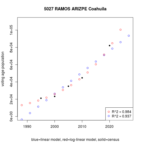
Figure 2 compares linear (in blue) and log-linear (in red) regression voting age population predictions against the censuses (in solid black). Regression projections do not match census points as segments did, but they summarize the central trend neatly—in most cases, at least. The log-tranformed approximates the Ramos Arizpe data more closely than the linear does, and this becomes clearer beyond the left and right census limits (1995 and 2020).

Table 2: Comparing the linear and log-linear models in two municipalities

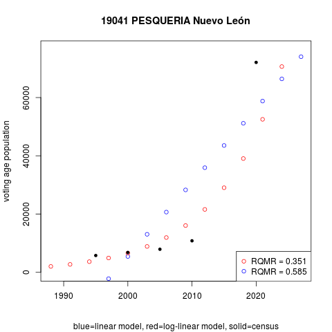Pesquería municipality in Nuevo León state is a case of extremely poor regression fit. Reached in the second half of the 2010s by Monterrey's dynamic suburban area, census data are highly volatile. Cases like this are present, but extremely rare. The table below reports regression models' quadratic mean of errors in census years. Quantities are divided by the municipio's mean voting age population in the period, thus expressing performance statistics as shares: a Relative Quadratic Mean Residual RQMR = 0.351 in Pesquería means that predictions are 35 percent off the census observations on average. Pesquería stands at the 99.96th percentile, among the bottom four hundredths percent with poorest fit.

Table 3: How far off are predictions in census years (as a share of the mean municipal population)?

Reverse percentile	worst	99%	95%	75%	50%	25%	5%	1%	best
Log linear projections	.355	.153	.082	.042	.027	.018	.010	.006	.002
Linear projections	.605	.178	.086	.042	.028	.019	.010	.006	.003

The table reveals comparatively similar performances of the linear and log-linear projections up about the 95th percentile. The log-linear bottom 5%, however, fared substantially better than the linear. This led me to choose it for extrapolation.

I perform off-census years projections using the following combination:

• Interpolation: for inter-census years, I rely on the segments model.
• Extrapolation: for years prior to the first census available and years after the latest census, I rely on log-linear regression predictions.

This combination can be seen in Figure 1. White circles are values segment-interpolated, exes mark log-linear-extrapolated values.

5 Projecting with three censuses only

A further obstacle for analysis is that the census bureau began distribution of sección-level census aggregates only in 2005.² So whereas five census points are available for municipal projections (six, when 1990 is added), there are three only for secciones: 2005, 2010, and 2020.

Extrapolation plays a limited role in municipal census projections. With five censuses to estimate from, they are needed for 1994 and 1991—both pre-competitive era elections that are often left aside—2021 and, soon, 2024. All are close to limit censuses, ensuring limited distortion in case inferred trends were off the mark. With three censuses only for secciones electorales, extrapolations are more in number an farther from the 2005 census. I gauge three-year projections in municipios. Having census points in 1995 and 2000 (unavailable for secciones) offers leverage to verify how far off from them land predictions made with 2005-2010-2020-only.

The experiment lends stronger support to the log-linear model. The table below gauges relative quadratic mean residuals in 1995 and in 2000 from linear and log-linear predictions made with 2005–2020 censuses only. RQMRs are not too different above the median, but patently diverge in the bottom half of the performance distributions, especially in more distant 1995. The log-linear 95th percentile voting age population prediction is 29 percent off its 1995 mean; the linear is off by 40 percent. By the 99th percentile, the linear divergence from target (132%) nearly triples the log-linear (55%).

Table 4: How far off are 3-year predictions in 1995 and 2000?

Reverse percentile	worst	99%	95%	75%	50%	25%	5%	1%	best
Log-linear 1995	1.881	.549	.290	.137	.074	.035	.006	.002	.000
Linear 1995	10.604	1.318	.404	.167	.092	.043	.010	.002	.000
Log-linear 2000	1.228	.511	.234	.101	.056	.026	.005	.001	.000
Linear 2000	5.185	.661	.250	.101	.052	.025	.005	.001	.000

Evaluation of other projection methods is desirable. Revise what demographers have written.

The procedure extends to other socio-demographic aggregate quantities.

6 References

Ponce López, Roberto. 2009. La geografía del voto en México: organización partidista en las secciones electorales, 1997–2003. Tesis de licenciatura, ITAM.

Evaluating Linearly Interpolated Intercensal Estimates of Demographic and Socioeconomic Characteristics of U.S. Counties and Census Tracts 2001–2009

Margaret M. Weden, Christine E. Peterson, Jeremy N. Miles & Regina A. Shih Population Research and Policy Review volume 34, pages541–559 (2015) –> pdf

Alexander Alkema 2021 –> pdf

Interpolating U.S. Decennial Census Tract Data from as Early as 1970 to 2010: A Longitudinal Tract Database John R. Logan,Zengwang Xu &Brian J. Stults Pages 412-420 Published online: 13 May 2014

Footnotes:

¹

INEGI replaced mid-decade `conteos' with a sample in 2015. Conteos Generales in 1995 and 2005 were a mini census, with a basic questionnaire excluding most items used in general censuses and with limited effort to re-interview non-responders. An opinion poll method was used instead in 2015, much cheaper yet hardly comparable. This note excludes the 1990 census, which needed cleaning. Repository projections include it.

²

Ponce (2009) attempted reconstruction of pre-2005 sección-level census data. The challenge is matching localidades (in rural Mexico) and manzanas (in urban Mexico), which INEGI has used as census tracts, to secciones electorales nationwide. Geo-referenced units open room to spot overlaps towards such match. It is worth revising his data.